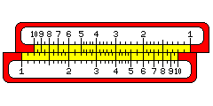
Since division using the C and D scales is simpler in practice than division using the CI scale and the D scale, it follows that multiplication might actually become simpler if the CI and D scales are used instead of the C and D scales.
In this diagram, we see that when a CI and D scale are slid together in contact, the product of the corresponding numbers on the scales is always the same:
10 * 1.2 = 8 * 1.5 = 6 * 2 = 4 * 3 = 3 * 4 = 2 * 6 = 1.5 * 8 = 1.2 * 10 = 12
So, to multiply, just bring the two numbers to be multiplied together, and then read the product at the index. This form of multiplication, with one additional wrinkle, as shown below,
was the one recommended for most duplex slide rules.
Let us say that it is desired to multiply 8 by 9. Instead of taking the 8 from one end of the CI scale, and the 9 from the opposite end of the D scale, a second set of folded scales, that is, scales starting at a different point from the usual one, is provided so that the rule needs to be moved only a short distance, across the index.
Since it is useful to be able to multiply quantities by pi, this is the value usually used for folded scales, although folding at the square root of 10 would bring the distance needed to move the rules to an absolute minimum.
Also, some slide rules had a DI scale in addition to the CI scale. Since the trig scales on a slide rule are usually on the slider, one thing having a DI scale facilitates is multiplications involving a trig function. It also provides more flexibility in ordinary multiplication and division.
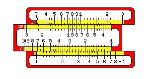
Here, below and to the left, is another, larger, and more realistic illustration of what a slide rule looked like than the one on the first page, which may prove useful as a reference to the discussion below.
We have seen how the C and D scales on a slide rule can be used to perform multiplication and division.
To multiply:
Place the index of the C scale over the multiplicand on the D scale; under the multiplier on the C scale, read the product on the D scale.
To divide:
Place the dividend on the C scale over the divisor on the D scale: over the index on the D scale, read the quotient on the C scale.
Each of these simple manipulations involves the use of the index. By using some other number in place of the index, it is possible to perform a multiplication and a division at the same time.
Thus, to solve the equation:
 x     q
--- = ---
 p     r
one can proceed as follows:
Place q on the C scale over r on the D scale.
Then, not only will the quotient, q/r, be found on the C scale over the index of the D scale, but every number on the C scale will be in the ratio of q/r to the number on the D scale below.
Thus, x will be found on the C scale over p on the D scale.
Of course, it certainly may happen that p on the D scale might be, for some values of q and r, beneath empty air. One way of dealing with this is to resort to the A and B scales, but the usual way of recovering is to move the cursor to that index of the C scale which is over a part of the D scale, and then, holding the cursor in place, moving the other index of the C scale to that point.
That is something that has to be done carefully to avoid losing accuracy, and thus the more advanced manipulations of the slide rule were not for everyone.
The fact that a typical slide rule does have A and B scales and a CI scale means that in the equation
 x     q
--- = ---
 p     r
any of the terms can be replaced by its square root. In the absence of both a CI scale and a DI scale, replacing terms by their reciprocals is not quite so arbitrary, but that is not a serious limitation since terms can also be shifted to different positions in the equation.
The fact that one has only a CI scale on the typical Mannheim rule, or only a DI scale on the front face of some duplex rules, can also mean, however, that one has to carefully plan which scale one uses as a starting point. It should be clear by now that it is for the purpose of faciltating this kind of slide rule manipulation, and not primarily for simple division and the taking of reciprocals, that CI or DI scales, as well as in some cases BI scales, are found on slide rules.
Recently, someone noted that a friend of his had a quick way to work out frequencies of resonant circuits on a slide rule, but did not reveal his secret.
The formula for the resonant frequency of a circuit involving an inductor and a capacitor is:
                 1
  f = -----------------------
                     _______
                    /
       2 * pi *    /  L * C
                 \/
Obviously, one can work this out in a step-by-step fashion on a slide rule; one might begin by using the A and B scales to multiply L by C, so that the square root of the product can be read off right away.
Doing that in the usual way, placing the index of the B scale under L on the A scale, and then moving the cursor to C on the B scale, lets one read L*C on the A scale, and sqrt(L*C) on the D scale.
At this point, an improvement suggests itself. If one is working with a slide rule with a CI scale and not a DI scale, starting by placing L on the B scale under the index of the A scale, and then continuing by moving the cursor to C on the A scale allows one not only to read L*C on the B scale, and sqrt(L*C) on the C scale, but also 1/sqrt(L*C) on the CI scale.
Since we began by using the index of the A scale (which, of course, coincides with the index of the D scale), can we shift our result along the CI scale so as to get our desired answer of 1/(2*pi*sqrt(L*C)) by starting with a different number? We certainly can, and what we need to start with is a point on the D scale rather than on the A scale, the number 1/(2*pi), which is about 0.159155. On a slide rule, of course, .159 is as precise as one needs get. As it happens, 10/(2*pi) cubed is 4.03144, so one can cheat a bit by using 4 on the K scale as an easy-to-remember starting point, although that does result in some real loss of accuracy, even within the limited precision of a slide rule.
In terms of the general equation given above, what we are doing is the calculation:
   1/x       sqrt(L)
--------- = ---------
 sqrt(C)    1/(2*pi)
where L and C both have their square roots substituted for them by using the B and A scales for them respectively, where 1/(2*pi) is simply a constant, and where 1/x is substituted for x by using the CI scale, rather than the C scale, to find x.
Some older manuals on the use of a slide rule provided a table of the possibilities afforded by the A, B, CI, C, and D scales. While it would be pointless, even in the heyday of the slide rule, for most users to try to memorize such a table, it certainly could be used as a reference if one wanted the quickest way to evaluate a particular simple formula.
While today such a table serves only to satisfy curiosity, or settle arguments, I still feel it sufficiently worthwhile to provide one.
In this table, p is always on the slider of the rule, and q is always on the body of the rule; r is on the slider or the body, and x is on the opposite portion of the rule. One begins by placing p in alignment with q, and then one finds x in alignment with r. For each combination of scales, the table shows what x is in terms of p, q, and r. Of course, there are many different combinations of scales that lead to equivalent results, but these are noted as well to make the table simple and uniform.
 p   q   r   x      x is equal to:     p   q   r   x      x is equal to:
-----------------------------------   -----------------------------------
 C   D   D   C      r * p/q            D   C   C   D      r * p/q
 C   D   D   CI     q/(p*r)            D   C   C   A      (r * p/q)^2
 C   D   D   B      (r * p/q)^2        D   C   CI  D      p/(q*r)
 C   D   A   C      sqrt(r) * p/q      D   C   CI  A      (p/(q*r))^2
 C   D   A   CI     q/(p*sqrt(r))      D   C   B   D      (p/q) * sqrt(r)
 C   D   A   B      r * (p/q)^2        D   C   B   A      r * (p/q)^2

 C   A   D   C      r * p/sqrt(q)      D   CI  C   D      p * q * r
 C   A   D   CI     sqrt(q)/(p*r)      D   CI  C   A      (p * q * r)^2
 C   A   D   B      (r * p)^2/q        D   CI  CI  D      p * q/r
 C   A   A   C      p * sqrt(r/q)      D   CI  CI  A      (p * q/r)^2
 C   A   A   CI     sqrt(q/r)/p        D   CI  B   D      p * q * sqrt(r)
 C   A   A   B      r * (p^2)/q        D   CI  B   A      r * (p*q)^2

 CI  D   D   C      r/(p * q)          D   B   C   D      r * p/sqrt(q)
 CI  D   D   CI     p * q/r            D   B   C   A      ((r * p)^2)/q
 CI  D   D   B      (r/(p * q))^2      D   B   CI  D      p/(r * sqrt(q))
 CI  D   A   C      sqrt(r)/(p * q)    D   B   CI  A      (p/r)^2 / q
 CI  D   A   CI     (p * q)/sqrt(r)    D   B   B   D      p * sqrt(r/q)
 CI  D   A   B      r/((p*q)^2)        D   B   B   A      p^2 * (r/q)

 CI  A   D   C      r/(p * sqrt(q))    A   C   C   D      r * sqrt(p)/q
 CI  A   D   CI     p * sqrt(q)/r      A   C   C   A      p * (r/q)^2
 CI  A   D   B      (r/p)^2/q          A   C   CI  D      sqrt(p)/(q*r)
 CI  A   A   C      sqrt(r/q)/p        A   C   CI  A      p/((q*r)^2)
 CI  A   A   CI     p*sqrt(q/r)        A   C   B   D      sqrt(p * r)/q
 CI  A   A   B      r/((p^2) * q)      A   C   B   A      r * p/(q^2)

 B   D   D   C      r * sqrt(p)/q      A   CI  C   D      q * r * sqrt(p)
 B   D   D   CI     q/(sqrt(p)*r)      A   CI  C   A      p * (q * r)^2
 B   D   D   B      p * (r/q)^2        A   CI  CI  D      q/r * sqrt(p)
 B   D   A   C      sqrt(r * p)/q      A   CI  CI  A      p * (q/r)^2
 B   D   A   CI     q/(sqrt(r * p))    A   CI  B   D      q * sqrt(p * r)
 B   D   A   B      r * p/(q^2)        A   CI  B   A      p * r * (q^2)

 B   A   D   C      r * sqrt(p/q)      A   B   C   D      r * sqrt(p/q)
 B   A   D   CI     sqrt(q/p)/r        A   B   C   A      (p/q) * r^2
 B   A   D   B      (r^2) * p/q        A   B   CI  D      sqrt(p/q)/r
 B   A   A   C      sqrt(r*p/q)        A   B   CI  A      p/(q*(r^2))
 B   A   A   CI     sqrt(q/(p * r))    A   B   B   D      sqrt(r * p/q)
 B   A   A   B      r * p/q            A   B   B   A      r * p/q
Although it isn't possible to trisect an angle using a straightedge and compasses when they are used in the standard way, performing the usual operations of drawing a straight line between two given points, or drawing a circle given its center and a point on its circumference, the ancient Greeks did know a way to trisect an angle by using these tools in a more creative way.
Of course, distinguishing the usual operations of geometrical construction from unusual ones was also very fruitful, since it led to a body of advanced mathematical theory.
The slide rule can also do some quite spectacular things if it is used in a somewhat analogous nonstandard fashion.
Let us move 1.1 on the B scale over 1 on the D scale.
Let us then move the cursor until the number on the B scale at the cursor is exactly one more than the number on the D scale at the cursor.
The result might be 1.508 on the D scale, and 2.508 on the B scale.
What problem has been solved?
The problem that was solved would be:
 1.1      x + 1
----- = ---------
   2         2
  1         x
If we cross-multiply, and then rearrange terms, we see that the equation we have solved is
1.1 x^2 - x - 1 = 0
Thus, the operation of sliding the cursor until the difference between the numbers on two scales reaches a desired value allows us to solve quadratic equations on the slide rule. Replacing 1.1 by some other number doesn't give us enough freedom to solve any quadratic equation, however; we can't just restrict ourselves to simple integer differences between the two scales to solve arbitrary quadratic equations, which does make this more difficult.
Placing a scale against an inverse scale, which can be done with an ordinary duplex slide rule by inverting the slider, which then places the CF scale, reversed, against the D scale, and the C scale, reversed, against the DF scale, lets one do something else remarkable with a slide rule rather more simply.
Since placing the index of one scale against a number on the other scale causes corresponding numbers along both scales to have that number as their product, the places where appropriate ticks coincide on both rules indicate factors of that number.
Performing addition in one's head, and then using the slide rule, can permit other complicated equations to be solved.
Let us place p on the B scale over p+q on the D scale.
Then, under q on the A scale, what do we find on the B scale?
The answer is that we find:
  2         2
 p + 2pq + q     p     q
------------- = --- + --- + 2
      pq         q     p
from which 2 can be subtracted mentally to produce a useful result.
Similarly, multiplying p+q by p-q produces p squared minus q squared; thus, doing so on the A and B scales can allow one to obtain the square root of p squared minus q squared on the C or D scale. A number of more complicated operations related to this one were devised by W. Ritter in 1894.
Adding and subtracting short numbers of the precision a slide rule can handle for multiplication, is trivial enough that normally it wouldn't seem worth the trouble to use a slide rule to help with that. But for completeness' sake, I thought it might be worthwhile to note how it can be dnne, at least theoretically.
Of course, if one had a second linear scale like the L scale, paired with it on the slider, one could use the slide rule to add easily, but this is a feature slide rules usually do not have. (One Pickett slide rule had something like that; it was connected with a feature for keeping track of the decimal point for beginning slide rule users.)
However, another method is possible.
If you have the logarithms of two numbers, x and y, if both are positive and y is less than x, log(x+y) = log(x) + log(1+y/x). Similarly, log(x-y) = log(x) + log(1-y/x).
It's easy to divide y by x on a slide rule.
But after one calculates y/x, doesn't one now need a new special scale on the slide rule to perform the addition?
Sort of. But here is what it would look like:

On the first line is the regular C scale of a slide rule; on the second line is the special scale needed for addition, and on the third line is the special scale needed for subtraction.
They look familiar, don't they?
Thus, the mental arithmetic of adding one to the ratio for addition, or subtracting the ratio from one for subtraction, is clearly trivial, and so no extra scales are needed.
For addition, only the part of the C scale going from 1 to 2 is needed; for subtraction, one may need multiple scales; so now instead of changing 1, 2, 3... 10 on C to .9, .8, .7,... 0, to get the next backward extansion, one changes them to .99, .98, .97,... .90 instead.
A concrete example may make the procedure clearer.
To add 1.65 and .85: first, divide .85 by 1.65, getting .515 as the answer. Since .85 is .515 of 1.65, then the sum of the two is 1.515 times 1.65, or 2.5 .