The Mollweide projection is an attempt to moderate the behavior of the equal-area sinusoidal projection.
It was originally invented in 1805 by Karl Mollweide, but Jacques Babinet independently re-invented it in 1857, and succeeded in making it well-known. Babinet also coined the term "homalographic", sometimes used to describe equal-area projections in general.
This projection is also equal-area. This is achieved by locating each parallel where the proportion of the area of the ellipse between that parallel and the equator is the same as the proportion of the area on the globe between that parallel and the equator.
This involves using iterative methods to determine the inverse of a function that cannot be inverted analytically, but the process converges rapidly.
Since a sinusoid takes up less space than an ellipse, there is some stretching of countries along the equator. Horizontal and vertical scales match at approximately 40° 44' 11.8" north and south, although only at the central meridian at that latitude is there no shape distortion.
Here is an old map drawn on the Mollweide projection:
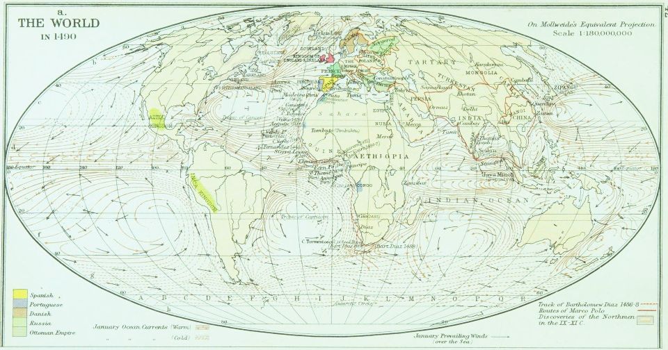
This map is from a historical atlas, published in 1927. It is interesting in that the realm of Tartary is shown on the map; some have said that Tartary is an old misnomer that lumped Turkestan and Mongolia together, but here both Turkestan and Mongolia are also shown on the map to the south of Tartary.
A strange pseudo-scientific notion has recently emerged that the civilization of Tartary was destroyed in a "mud flood" but that they left behind bridges that were built in mediaeval times and were far advanced of their time... which are now cunningly disguised as bridges of modern construction.
At least you can still buy Tartar sauce at the supermarket.
Since this projection is a pseudocylindrical projection like the Sinusoidal projection, it can be interrupted.
The interrupted Mollweide dates back to 1916, originally proposed, along with the interrupted Sinusoidal, by J. Paul Goode, who, later, in 1923, came up with the Goode Homolosine projection, which switched from the Sinusoidal to the Mollweide so as to use the Sinusoidal for equatorial regions, where it had less distortion, but the Mollweide for polar regions, where it avoided extreme shear.
And, like any projection, it can be drawn in its oblique case:
Since it presents the world on an ellipse, doing so with the Mollweide is more popular than with the Sinusoidal projection, although the Hammer-Aitoff projection has proved even more popular for versions of the projection in an oblique aspect.
But there is one famous version of the Mollweide projection in a transverse aspect that was widely used for a time:
This is Bartholomew's Atlantis projection, devised by John Ian Bartholomew, C. B. E., M. C., LL. D. (1890-1962).
Because the Mollweide projection stretches the area around the Equator, and has standard parallels near 40 degrees of latitude on both sides of the Equator, aspects that place the areas of maximum interest in the center of the map are better done on the Hammer-Aitoff projection. The Atlantis projection, on the other hand, is an aspect that makes good use of the Mollweide, since the most important land areas are in the areas of low distortion, with the equatorial stretching dumped in the middle of the Atlantic Ocean.
Here is a diagram, drawn by the program Flex Projector, showing how angular distortion is distributed on the Mollweide projection in order to make this clear:
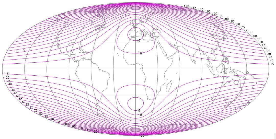
Unfortunately, I've had to choose one on a somewhat large scale so that the central area of low distortion is clearly identifiable.
A more conventional method of acknowledging the distribution of distortion in the Mollweide projection was used by the Soviet cartographer Solovev in 1946:
which tilts the map forwards, like Bartholemew's Nordic projection, but, because the Mollweide instead of the Hammer-Aitoff projection is used, tilts the globe by a lesser amount to put Europe in the area of minimum distortion.
However, given what that projection does to the area around the Bering Strait, perhaps instead of being intended for a world map, it was merely intended for a map of the Soviet Union, as illustrated here:
On the other hand, for a projection in this kind of aspect, the difference in the distribution of distortion between the Hammer-Aitoff and the Mollweide may not be too much of an issue. In the book World Maps and Globes by Irving Fisher and Osborn Maitland Miller, in 1944, the following oblique Mollweide appeared:
in precisely the same orientation that would later be used with the Hammer-Aitoff in 1948 by John Ian Bartholomew in his Nordic projection.
Incidentally, the book World Maps and Globes was likely the first book to mention Adams' conformal projection of the world on an ellipse to a general audience.
Before I saw that, I had found an image online of the Geographia New Standard World Atlas from the Geographia Map Company, in the United States, dated 1947, with this projection on the cover:
Still with the Prime Meridian in the center, it differs from both the projection appearing in World Maps and Globes and Bartholomew's Nordic Projection in being tilted 40 degrees forwards rather than 45.
Initially, I thought this had been on the Hammer-Aitoff projection, and showed that Bartholomew had been anticipated, but a close look at the picture on the cover showed Europe was considerably stretched, meaning that it was the Mollweide that had been used.
A Transverse Mollweide, but in the Second Transverse aspect, instead of the Transverse Oblique aspect, and not taking advantage of the low-distortion regions of the Mollweide in the adroit way the Atlantis projection does, appeared in the 1912 book Map Projections by Arthur R. Hinks; it was credited to Colonel Sir Charles Close, its inventor. The Hammer-Aitoff projection is also described in that book, but it is referred to as Aitoff's projection - an error I believe to have been quite common, with Aitoff's actual projection, based on the Azimuthal Equidistant, being obscure until recently.
Above is the aspect of the Mollweide devised by Sir Close; but he is also associated with an oblique aspect of it as well:
In fact, this projection was originally proposed by J. Fairgrieve in 1928, and Close published a paper, crediting him, in which he described this projection, which explains why my original source credited him instead of Fairgrieve.
While this aspect places part of Asia on the edge of the map, where it is highly distorted, it did put nearly all the lands of the British Empire in an advantageous position, and even India was still recognizable.
Also, it should not be forgotten that it is possible
to combine the advantages of an interrupted projection with the advantages of an oblique aspect of the projection.
As it may sometimes be difficult to tell what is going on in an interrupted oblique projection, I feel it will be helpful to supply this explanatory diagram:
The upper portion of the diagram consists of this interrupted oblique projection, with the sections using the five different central meridians color coded, and the central meridians, as well as the equator, of the projection drawn in red.
The lower portion of the diagram shows a map of the world on a cylindrical projection (the Miller Cylindrical, in this case) obliqued in the same manner as used for this interrupted oblique Mollweide, and overlaid with a conventional graticule in red.
Triangles, bearing the colors used for color-coding the segments of the projection in the top part of the diagram, indicate the value of each central meridian in projection-native coordinates.
The diagram below illustrates the mathematical theory behind the Mollweide projection.
The Cylindrical Equal-Area projection illustrates the fact that the proportion of the Earth's surface area between a given latitude and the Equator is proportional to one-half the sine of the latitude.
Simple geometry shows what the proportion of the area of a circle is between a diameter and a line parallel to the diameter. In the diagram, it is expressed in terms of the angle psi rather than the height of the second line, for simplicity. The green triangular areas each have an area of sin(psi)*cos(psi)/2, and the yellow portions of the circle each have an area of psi/2. The circle as a whole has an area of pi.
Since the Mollweide projection places the world in an ellipse, the same proportionality law applies to the area between its parallels and the Equator.
The expression for this area, though, cannot be inverted simply. However, an iterative process can quickly determine the proper value for psi (from which the height can be directly calculated, as it is the sine of psi). Since the expression can be easily differentiated, instead of using a binary search, one can use Newton-Raphson iteration, which converges very quickly.
That is, to solve the equation:
(psi+sin(psi)cos(psi))/pi = sin(lat)/2
for psi, given lat, one can start with lat as our first guess for psi, and then improve each guess by noting that the difference between the true area and that given by any guess is:
error = ((guess+sin(guess)cos(guess))/pi - sin(lat)/2)
and, since the rate of change in that area for a change in the guess is the following function:
(1+(cos(guess))^2-(sin(guess))^2)/pi
then a good next guess is the old guess minus the error divided by the rate of change in the error over the rate of change in the guess.
The areas along the Equator in the Mollweide projection are stretched vertically. How much are they stretched by? That is a question that can be answered by some simple mathematics.
On the Sinusoidal projection, which is also twice as wide as it is high, the height of areas along the Equator is accurate. So the amount of stretching, which increases areas as well as heights, must equal the ratio in area between a circle (or ellipse) and the sinusoid within.
In the diagram above, we see a circle; let's assume its radius is 1.
The area of a circle is pi r squared, pi * r^2, so the area of this circle, then, is pi.
The area of the diagonal square is 2, since its diagonal sides have the square root of 2 as their length, given that they're diagonals of squares of side 1 having the center of the circle as one of their corners.
So the area of the sinusoid is some number between 2 and pi (3.141592653589793...). But what is it, exactly?
The diagram below will help us figure that out.
In the top half of the diagram, we see an illustration of the trigonometric sine function and its definition. As the red line sweeps out in counter-clockwise motion from the horizontal, the height of the point at which it intersects the circle is the sine of the angle it makes with the horizontal.
So the graph of the sine function... is a sinusoid.
What is the area of a sinusoid? Well, the area under a line on a graph is the integral of the function being graphed. And an integral is an antiderivative, from the Fundamental Theorem of Calculus.
The Fundamental Theorem of Calculus can be derived from the fact that when you are paintng a fence, you use your paint up twice as fast in parts of the fence that are twice as high.
The derivative of the sine is the cosine: this can be determined by the fact that when you walk around in circles, the direction you are facing also turns around in a circle if you're facing forwards.
A more illustrative explanation of these facts, such as might be found in an introductory calculus textbook, will be put aside for now.
In any case, the derivative of the cosine in turn is minus the sine.
Integrals aren't just antiderivatives. Since the area under a portion of a graph of length zero is always zero, as long as the function is finite, there is also a constant term reflecting where you're starting from.
So the definite integral of the sine of an angle, starting from zero, isn't just minus the sine of the ending angle, it's minus the sine of the ending angle plus one.
So the area of a curve that looks like half our sinusoid above is equal to 2, so the area of the sinusoid is 4.
Hey, wait a moment, that's bigger than pi! Not so fast! That's the area of a sinusoid with a width of 2 and a height of pi! So we have to scale it down, since the sinusoid of which we want the area has a width of 2 and a height of 2.
So we start with 4, but then we divide it by pi/2, so we get 8/pi, which is 2.54647908947..., and which is indeed a number between pi and 2, just like we wanted.
And the stretching factor is pi divided by this number, or pi^2 over 8, or 1.23370055..., so we have the answer we wanted.
The Wagner IV or Putniņš P2' projection is a modification of the Mollweide projection. Instead of using the whole ellipse, only the area up to where the ellipse is half as wide as it is at the equator is used to represent the Earth, The map is stretched vertically so that it remains half as high as it is wide. The latitude can be transformed using two superposed equal-area cylindrical projections, and then a Mollweide projection calculated, and then the final result stretched, or a modified iteration can be performed directly.
The vertical stretch is clearly the reciprocal of the cosine of 30 degrees, or approximately 1.15470053837925, and the factor by which one reduces the sine of the latitude is the ratio of the area of a circle with unit radius, which is pi, to two-thirds pi plus the cosine of 30 degrees, the area of a circle with two one-sixth pie-slices replaced by equilateral triangles, which is a factor of about 0.9423311143775627.
This leads to the Wagner IV projection, as pictured above.
If the vertical stretch given above is omitted, the result is the Werenskiold III projection.
On the page about the Gall Sterographic projection, I note that I tend to prefer projections which don't stretch shapes at the Equator, and the Braun projection was a modification of the Gall projection that had correct scale at the Equator. The same can be done with the Mollweide, and the result is the Bromley-Mollweide projection:
One useful application of this would be for an interrupted projection, where the Northern hemisphere is shown on the Bromley projection with only a limited number of interruptions, while the Southern hemisphere is shown on a Sinusoidal projection with multiple interruptions. An example of this is shown below:
With an oblique projection, one can avoid the need to interrupt the Northern hemisphere at all, and obtain something more strongly reminiscent of the famous Sinu-Mollweide projection by Philbrick:
Speaking of Philbrick's Sinu-Mollweide, I would be remiss if I did not mention one of the most famous developments of the Mollweide projection:
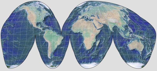
Goode's Homolosine projection, shown above in a rendering provided by G.Projector.
An ellipse of a given width is larger in area than a sinusoid of that width; if the Mollweide projection and the Sinusoidal projection are drawn to the same scale in area, the latitude at which they will have the same width is the one where the Mollweide is conformal on its central meridian: approximately 40° 44′ 12″.
The idea behind it is to avoid the extreme distortion of the Sinusoidal projection near the poles, while also avoiding the stretching of the Mollweide projection in equatorial regions. The price which it pays, which in my opinion is too heavy to be borne, is that at the latitude where the two projections are joined, there is a sudden kink in the map. Even if the kink is a small one, and hardly visible at the scale of the illustration above.